

7 Amazing Tips & Tricks in Excel
- Admin

- Mar 5, 2018
- 4 min read
1. Entering Line Sparkline Microcharts
Line Sparklines are mini charts placed in single cells, each representing a row of data in your selection. This could be used to show the trends of multiple items together. This enhance the view and helps in understanding the trends. To make one, you need to first select the data from which you wish to create a sparkline, and then go to Inset ->Line.

There you will be asked to enter the destination location of your sparkline chart. Select the destination location to draw the Sparkline chart. Once you are done, you can see amazing sparkline chart ready.

2. Conditional formatting
This is one of the magical Excel built-in features that I often use to prepare dashboard or management reports. It’s very simple to use, however, one can customize as per their need in order to get the maximum benefit.
Getting back to our previous table, Select the column on which you want to apply the conditional formatting

As you can see, there are lot of options that we can use but I’ll try to cover options which I find enough to prepare excellent reports. No doubt once can go beyond the limit by exploring features.
There are 3 easy to use feature in conditional formatting:
Data Bar
Color Scales
Icon Set
1. Data Bar: It is used to represent the value in the cell. Higher the value, longer the bar.

2. Color Scale: Apply the color gradients to a range of cells, color indicates where each value falls within that range.
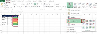
3. Icon set: It is used to represent values in cells through icons.

Are you impressed with this feature? If Yes then hold on – as there are some more magical feature available that you can use very easily.
You can select “More Rules” to customize the indicator to suit your need.

(It can be done for data bar and color scales also) Once you click on More Rules, you will see the form to customize the indicators.

3. VLOOKUP
VLOOKUP is one of the powerful feature offered by Excel and I’m sure most of you already aware of it. Formula format for the VLOOKUP is as below:
VLOOKUP (Lookup value, table array, col_index_num, [range lookup])
Lookup value: The value to search for in the first column of the table.
Table array: Two or more columns of data that are sorted in ascending order.
Col_index_num: The column number in the table from which the matching value must be returned. The first column is 1.
[Range lookup]: Optional. Enter FALSE to find an exact match. Enter TRUE to find an approximate match. If this parameter is omitted, TRUE is the default.
Note:
If you specify FALSE for the approximate_match parameter and no exact match is found, then the VLOOKUP function will return #N/A.
If you specify TRUE for the approximate_match parameter and no exact match is found, then the next smaller value is returned.
If index_number is less than 1, the VLOOKUP function will return #VALUE!.
If index_number is greater than the number of columns in table, the VLOOKUP function will return #REF!.
Example: Let’s go back to our first table (let’s call it Table A) which has name, age and Rank details. I have created on more table (Let’s call it Table B) with department and its fixed basic salary. Now, I will add two columns i.e. Department, Salary in table A and I will write vlookup formula on Salary column to get the salary from Table A based on department selected in column D.

You can also use the various charting option available in excel to showcase the data in the pictorial form.
4. Move and Copy Data in Cells Quickly
If you want to move a column data quickly then you can simply select the column and point the mouse cursor to the column border and drag freely to required place.

However, you can also quickly copy and paste the selected column by just pressing Ctrl while dragging the column.

It was quick isn’t it?
5. Generate a Unique Value in a Column
Sometimes you may need to filter the unique values from the repeated data and it can be easily done by using excel inbuilt feature.
Steps to filter unique values from the repeated data:
Go to Data -> Advance Filter

You can filter unique values in the same column by selecting “Filter the list – In place” or filter the record in different column by selecting “Copy to another location”

Note: Don’t forget to select “Unique records only”.
6. Input Restriction with Data Validation Function
Sometimes you may need to restrict values in the column in order to maintain the validation. For an example, in below table, I don’t want the age of the person to be less than 20 or greater than 50.
Follow the below steps to put data validation to your column
Select the column and go to Data ->Data Validation

Select the minimum and maximum values, Validation Message and Error Alert for customized error.

Result:

Note: You can explore more by selecting different values in Allow and Data drop-down.
7. Transpose Data from a Row to a Column
This feature can be used when you want to transpose the data for better display or any other purpose. This is very cool feature as you don’t need to retype the data.
Follow the below steps…
Copy the complete table which you want to transpose.

Go to Paste – > Transpose (You can also Right Click – > Paste Options – > Transpose)

Result:

Note: Function will only be available once you copy the data.
Hope you liked this article, If you have any Excel trick that could be useful in day to day work then please share in the comment section. You can also share these tricks with your friends by using share button.
Reference: buzzanalysis.com


Comments